 1
 2
 3
 4
 5
 6
 7
 8
 9
10
11
12
13
14
15
16
17
18
19
20
21
22
23
24
25
26
27
28
29
30
31
32
33
34
35
36
37
38
39
40
41
42
43
44
45
46
47
48
49
50
51
52
53
54
55
56
57
58
59
60
61
62
63
64
65
66
67
68
69
70
71
72
73
74
75
76
77
78
79
80
81
82
83
84
85
86
87
88
89
90
91
92
93
94
95
96
97
98
99
100
101
102
103
104
105
106
107
108
109
110
111
112
113
114
115
116
117
118
119
120
121
122
123
124
125
126
127
128
129
130
131
132
133
134
135
136
137
138
139
140
141
142
143
144
145
146
147
148
149
150
151
152
153
154
155
156
157
158
159
160
161
162
163
164
165
166
167
168
169
170
171
172
173
174
175
176
177
178
179
180
181
182
183
184
185
186
187
188
189
190
191
192
193
194
195
196
197
198
199
200
201
202
203
204
205
206
207
208
209
210
211
212
213
214
215
216
217
218
219
220
221
222
223
224
225
226
227
228
229
230
231
232
233
234
235
236
237
238
239
240
241
242
243
244
245
246
247
248
249
250
251
252
253
254
255
256
257
258
259
260
261
262
263
264
265
266
267
268
269
270
271
272
273
274
275
276
277
278
279
280
281
282
283
284
285
286
287
288
289
290
291
292
293
294
295
296
297
298
299
300
301
302
303
304
305
306
307
308
309
310
311
312
313
314
315
316
317
318
319
320
321
322
323
324
325
326
327
328
329
330
331
332
333
334
335
336
337
338
339
340
341
342
343
344
345
346
347
348
349
350
351
352
353
354
355
356
357
358
359
360
361
362
363
364
365
366
367
368
369
370
371
372
373
374
375
376
377
378
379
380
381
382
383
384
385
386
387
388
389
390
391
392
393
394
|
"""
Suppose you are the product manager of the factory and you have the test results for some microchips on two different tests.

From these two tests, you would like to determine whether the microchips should be accepted or rejected.
To help you make the decision, you have a dataset of test results on past microchips, from which you can build a logistic regression model.

"""

import numpy as np
import matplotlib.pyplot as plt
from utils import *
import copy
import math


def cat_data():
    # Plot examples
    plot_data(X_train, y_train[:], pos_label="Accepted", neg_label="Rejected")

    # Set the y-axis label
    plt.ylabel('Microchip Test 2')
    # Set the x-axis label
    plt.xlabel('Microchip Test 1')
    plt.legend(loc="upper right")
    plt.show()


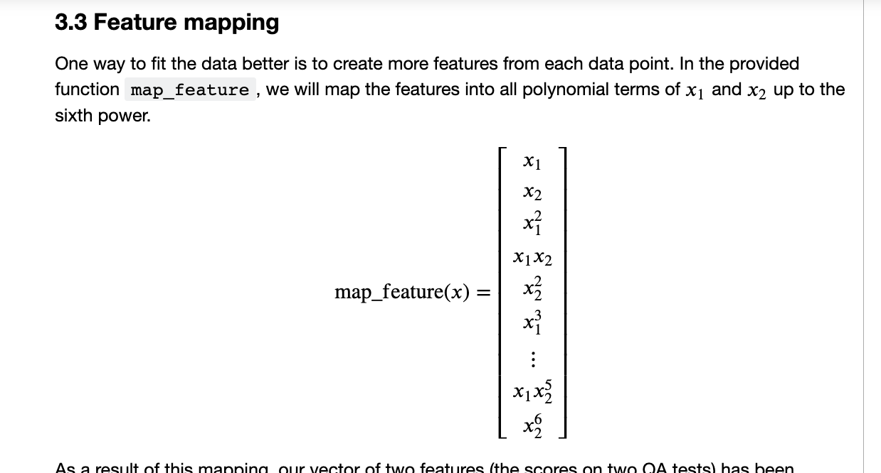
def map_feature(X1, X2):
    """
    Feature mapping function to polynomial features
    we will map the features into all polynomial terms of  𝑥1  and  𝑥2  up to the sixth power.
    """
    X1 = np.atleast_1d(X1)
    X2 = np.atleast_1d(X2)
    degree = 6
    out = []
    for i in range(1, degree+1):
        for j in range(i + 1):
            out.append((X1**(i-j) * (X2**j)))
    return np.stack(out, axis=1)


# UNQ_C1
# GRADED FUNCTION: sigmoid

def sigmoid(z):
    """
    Compute the sigmoid of z

    Args:
        z (ndarray): A scalar, numpy array of any size.

    Returns:
        g (ndarray): sigmoid(z), with the same shape as z

    """

    ### START CODE HERE ###
    g = 1 / (1 + np.exp(-z))

    ### END SOLUTION ###

    return g

# UNQ_C2
# GRADED FUNCTION: compute_cost
def compute_cost(X, y, w, b, lambda_=1):
    """
    Computes the cost over all examples
    Args:
      X : (ndarray Shape (m,n)) data, m examples by n features
      y : (array_like Shape (m,)) target value
      w : (array_like Shape (n,)) Values of parameters of the model
      b : scalar Values of bias parameter of the model
      lambda_: unused placeholder
    Returns:
      total_cost: (scalar)         cost
    """

    m, n = X.shape

    ### START CODE HERE ###
    loss_sum = 0

    # Loop over each training example
    for i in range(m):
        # First calculate z_wb = w[0]*X[i][0]+...+w[n-1]*X[i][n-1]+b
        z_wb = 0
        # Loop over each feature
        for j in range(n):
            # Add the corresponding term to z_wb
            z_wb_ij = w[j] * X[i][j]  # Your code here to calculate w[j] * X[i][j]
            z_wb += z_wb_ij  # equivalent to z_wb = z_wb + z_wb_ij
        # Add the bias term to z_wb
        z_wb += b  # equivalent to z_wb = z_wb + b

        f_wb = sigmoid(z_wb)  # Your code here to calculate prediction f_wb for a training example
        # ?
        loss = -y[i] * np.log(f_wb) - (1 - y[i]) * np.log(
            1 - f_wb)  # Your code here to calculate loss for a training example

        loss_sum += loss  # equivalent to loss_sum = loss_sum + loss

    total_cost = (1 / m) * loss_sum
    ### END CODE HERE ###

    return total_cost


# UNQ_C5
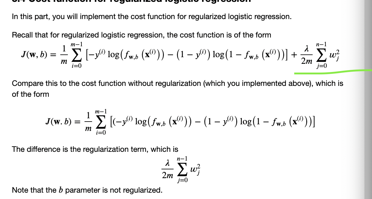
def compute_cost_reg(X, y, w, b, lambda_=1):
    """
    计算正则项
    Computes the cost over all examples
    Args:
      X : (array_like Shape (m,n)) data, m examples by n features
      y : (array_like Shape (m,)) target value
      w : (array_like Shape (n,)) Values of parameters of the model
      b : (array_like Shape (n,)) Values of bias parameter of the model
      lambda_ : (scalar, float)    Controls amount of regularization
    Returns:
      total_cost: (scalar)         cost
    """

    m, n = X.shape

    # Calls the compute_cost function that you implemented above
    cost_without_reg = compute_cost(X, y, w, b)

    # You need to calculate this value
    reg_cost = 0.

    ### START CODE HERE ###
    for j in range(n):
        reg_cost_j = w[j] ** 2  # Your code here to calculate the cost from w[j]
        reg_cost = reg_cost + reg_cost_j

    ### END CODE HERE ###

    # Add the regularization cost to get the total cost
    total_cost = cost_without_reg + (lambda_ / (2 * m)) * reg_cost

    return total_cost


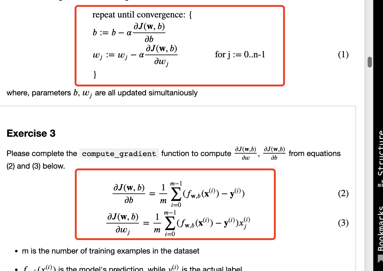
def compute_gradient(X, y, w, b, lambda_=None):
    m, n = X.shape
    dj_dw = np.zeros(w.shape)
    dj_db = 0.

    ### START CODE HERE ###
    err = 0.
    for i in range(m):
        # Calculate f_wb (exactly as you did in the compute_cost function above)
        z_wb = 0
        # Loop over each feature
        for j in range(n):
            # Add the corresponding term to z_wb
            z_wb_ij = X[i, j] * w[j]
            z_wb += z_wb_ij

        # Add bias term
        z_wb += b

        # Calculate the prediction from the model
        f_wb = sigmoid(z_wb)

        # Calculate the  gradient for b from this example
        dj_db_i = f_wb - y[i]  # Your code here to calculate the error

        # add that to dj_db
        dj_db += dj_db_i

        # get dj_dw for each attribute
        for j in range(n):
            # You code here to calculate the gradient from the i-th example for j-th attribute
            dj_dw_ij =(f_wb - y[i])* X[i][j]
            dj_dw[j] += dj_dw_ij

    # divide dj_db and dj_dw by total number of examples
    dj_dw = dj_dw / m
    dj_db = dj_db / m
    ### END CODE HERE ###

    return dj_db, dj_dw


# UNQ_C6
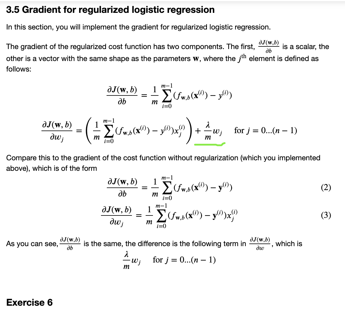
def compute_gradient_reg(X, y, w, b, lambda_=1):
    """
    Computes the gradient for linear regression

    Args:
      X : (ndarray Shape (m,n))   variable such as house size
      y : (ndarray Shape (m,))    actual value
      w : (ndarray Shape (n,))    values of parameters of the model
      b : (scalar)                value of parameter of the model
      lambda_ : (scalar,float)    regularization constant
    Returns
      dj_db: (scalar)             The gradient of the cost w.r.t. the parameter b.
      dj_dw: (ndarray Shape (n,)) The gradient of the cost w.r.t. the parameters w.

    """
    m, n = X.shape

    dj_db, dj_dw = compute_gradient(X, y, w, b)

    ### START CODE HERE ###
    for j in range(n):
        dj_dw_j_reg = (lambda_ / m) * w[j]
        dj_dw[j] = dj_dw[j] + dj_dw_j_reg

    ### END CODE HERE ###

    return dj_db, dj_dw


def gradient_descent(X, y, w_in, b_in, cost_function, gradient_function, alpha, num_iters, lambda_):
    """
    Performs batch gradient descent to learn theta. Updates theta by taking
    num_iters gradient steps with learning rate alpha

    Args:
      X :    (array_like Shape (m, n)
      y :    (array_like Shape (m,))
      w_in : (array_like Shape (n,))  Initial values of parameters of the model
      b_in : (scalar)                 Initial value of parameter of the model
      cost_function:                  function to compute cost
      alpha : (float)                 Learning rate
      num_iters : (int)               number of iterations to run gradient descent
      lambda_ (scalar, float)         regularization constant

    Returns:
      w : (array_like Shape (n,)) Updated values of parameters of the model after
          running gradient descent
      b : (scalar)                Updated value of parameter of the model after
          running gradient descent
    """

    # number of training examples
    m = len(X)

    # An array to store cost J and w's at each iteration primarily for graphing later
    J_history = []
    w_history = []

    for i in range(num_iters):

        # Calculate the gradient and update the parameters
        dj_db, dj_dw = gradient_function(X, y, w_in, b_in, lambda_)

        # Update Parameters using w, b, alpha and gradient
        w_in = w_in - alpha * dj_dw
        b_in = b_in - alpha * dj_db

        # Save cost J at each iteration
        if i < 100000:  # prevent resource exhaustion
            cost = cost_function(X, y, w_in, b_in, lambda_)
            J_history.append(cost)

        # Print cost every at intervals 10 times or as many iterations if < 10
        if i % math.ceil(num_iters / 10) == 0 or i == (num_iters - 1):
            w_history.append(w_in)
            print(f"Iteration {i:4}: Cost {float(J_history[-1]):8.2f}   ")

    return w_in, b_in, J_history, w_history  # return w and J,w history for graphing


def predict(X, w, b):
    """
    Predict whether the label is 0 or 1 using learned logistic
    regression parameters w

    Args:
    X : (ndarray Shape (m, n))
    w : (array_like Shape (n,))      Parameters of the model
    b : (scalar, float)              Parameter of the model

    Returns:
    p: (ndarray (m,1))
        The predictions for X using a threshold at 0.5
    """
    # number of training examples
    m, n = X.shape
    p = np.zeros(m)

    ### START CODE HERE ###
    # Loop over each example
    for i in range(m):
        z_wb = 0
        # Loop over each feature
        for j in range(n):
            # Add the corresponding term to z_wb
            z_wb += X[i, j] * w[j]

        # Add bias term
        z_wb += b

        # Calculate the prediction for this example
        f_wb = sigmoid(z_wb)

        # Apply the threshold
        p[i] = f_wb >= 0.5

    ### END CODE HERE ###
    return p


def plot_decision_boundary(w, b, X, y):
    # Credit to dibgerge on Github for this plotting code

    plot_data(X[:, 0:2], y)

    if X.shape[1] <= 2:
        plot_x = np.array([min(X[:, 0]), max(X[:, 0])])
        plot_y = (-1. / w[1]) * (w[0] * plot_x + b)

        plt.plot(plot_x, plot_y, c="b")

    else:
        u = np.linspace(-1, 1.5, 50)
        v = np.linspace(-1, 1.5, 50)

        z = np.zeros((len(u), len(v)))

        # Evaluate z = theta*x over the grid
        for i in range(len(u)):
            for j in range(len(v)):
                z[i, j] = sig(np.dot(map_feature(u[i], v[j]), w) + b)

        # important to transpose z before calling contour
        z = z.T

        # Plot z = 0
        plt.contour(u, v, z, levels=[0.5], colors="g")


if __name__ == '__main__':
    # X_train contains the test results for the microchips from two tests
    # y_train contains the results of the QA
    X_train, y_train = load_data("data/ex2data2.txt")

    # cat_data()

    print("Original shape of data:", X_train.shape)

    mapped_X = map_feature(X_train[:, 0], X_train[:, 1])
    print("Shape after feature mapping:", mapped_X.shape)

    # print("X_train[0]:", X_train[0])
    # print("mapped X_train[0]:", mapped_X[0])
    X_mapped = map_feature(X_train[:, 0], X_train[:, 1])
    np.random.seed(1)
    initial_w = np.random.rand(X_mapped.shape[1]) - 0.5
    initial_b = 0.5
    lambda_ = 0.5
    cost = compute_cost_reg(X_mapped, y_train, initial_w, initial_b, lambda_)

    print("Regularized cost :", cost)

    X_mapped = map_feature(X_train[:, 0], X_train[:, 1])
    np.random.seed(1)
    initial_w = np.random.rand(X_mapped.shape[1]) - 0.5
    initial_b = 0.5

    lambda_ = 0.5
    dj_db, dj_dw = compute_gradient_reg(X_mapped, y_train, initial_w, initial_b, lambda_)

    print(f"dj_db: {dj_db}", )
    print(f"First few elements of regularized dj_dw:\n {dj_dw[:4].tolist()}", )

    # Initialize fitting parameters
    np.random.seed(1)
    initial_w = np.random.rand(X_mapped.shape[1]) - 0.5
    initial_b = 1.

    # Set regularization parameter lambda_ to 1 (you can try varying this)
    lambda_ = 0.01
    # Some gradient descent settings
    iterations = 10000
    alpha = 0.01

    w, b, J_history, _ = gradient_descent(X_mapped, y_train, initial_w, initial_b,
                                          compute_cost_reg, compute_gradient_reg,
                                          alpha, iterations, lambda_)


    #Compute accuracy on the training set
    p = predict(X_mapped, w, b)

    print('Train Accuracy: %f'%(np.mean(p == y_train) * 100))
|


